April 11 – 18

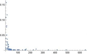
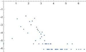
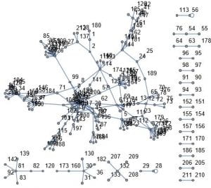
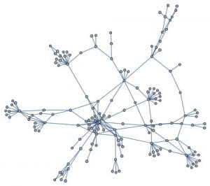
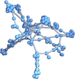
This week I decided to work on a random duplication network. I start with a graph of a ppi network 1 – 20 vertices. I then pick at random a vertex to duplicate. In my case the random choice was 12. I then join this vertex to 11 and 13. I add these new edges to the original network. I do this many times. After doing this 160 times this is the result.

April 4 – 11

This week I have decided to focus on a scale free networks. I load the ppi network that professor Davis has provided in the class notes into Mathematica. To figure out if a ppi network is scale free you have to construct a table of p(k) versus k. You then have to plot the log of P(k) and the log of k. If the plot shows a straight line then it is a scale free network.
This is a table of P(k) versus k. Lets see a graph of log(P(k)) and log(k).

From this plot we can see there is no straight line meaning this is not a scale free network.

March 27-April 3

This week I decided to replicate what we learned in the PPI network lecture. I first loaded the protein to protein data into Mathematica, (after great difficulty unzipping the file). After I imported the data I made a graph.

This is a graph of all the connections between the various proteins. We can see that there appears to be some clusters. One big cluster and several smaller clusters. We should plot the bigger cluster separately on another graph.

Here is a 3d version of the same graph.

Next week I would like to do something similar but with another PPI dataset.

Week of feb 14

This week I decided to do spacial visualization on a smaller species of plant. A couple weeks ago I did the same thing to the second most number of plant species. This was the result.

This was the result of doing the same visualization on the plant species “parodychia jamesii”

We can see that there is less data points, which reveals that the way the plants are positioned is not random. It got a chi squared statistic of 0, which means the way the plants are positioned is not random.

Week of feb 7

This week I didn’t make a lot of progress. I would have liked to do a visualization on a species with less numbers of instances. I have done visualizations on the biggest and second biggest species and have gotten inconclusive results. If I did the same procedures on a smaller species maybe I would get better results.

week of jan 31

In class we learned how to test for complete spacial randomness with the plant species with the largest amount of plants. I wanted to do this with another plant species. I took the second largest plant species and I plotted all the occurrences of the plant.

At first glance this looks random. Lets see if it is distributed randomly. To do this we need to test for a homogeneous Poisson distribution. I divided up the model into 10,000 pieces and check for the chi squared statistic. I got a chi squared probability of 1.9 * 10^-57, a very small probability. The data fits a Poisson distribution very poorly.

Week of jan 17

In class this week we organized the data about plants in Kansas into a Pareto curve. This week I decided to do more with this Pareto curve. The Pareto curve is named after Vilfredo Pareto who observed that 80% of the wealth is concentrated in the hands of 20% of the population. The Pareto principle states that 80% of outcomes are due to 20% of causes. I wanted to see if that was true for this data.

This was not true. Only 5 species caused 80% of cases out of a total number of 149 plant species. A value of only 3%.